Full Hypercausal System Demo (PennyLane + SPSA + KL)#

Overview#

This example demonstrates a full hypercausal system on a PennyLane backend, combining causal feedback with SPSA derivative-free optimization and a KL-constrained trust-region guard. Dynamic depth scheduling and multi-metric telemetry track how the internal feedback parameter \(\alpha\) co-evolves with coherence and consistency under non-stationary drift.

The model evaluates the stability of quantum-inspired feedback systems under drift, using adaptive control of internal causal parameters to maintain temporal coherence and counterfactual consistency.

Core Objectives#

Hypercausal Feedback Modeling: multi-directional causal propagation.
Quantum-Inspired Efficiency: simulated superposition for reduced cost.
Deterministic–Stochastic Integration: deterministic and probabilistic backends.
Causal Stability Measurement: tracking coherence, consistency, and feedback drift.
Scientific Transparency: reproducible, open experimentation.

Experimental Setup#

We simulate a minimal quantum-like node structure using PennyLane circuits. The internal state \(S_t\) evolves via recursive updates modulated by a causal feedback coefficient \(\alpha\), representing the degree of self-consistent causal correction.

The environment introduces a small non-stationary drift (sinusoidal) to evaluate robustness of the feedback mechanism.

System Architecture & Modules#

This demo wires the high-level components of QML-HCS as follows:

Backend: PennyLaneBackend with BackendConfig(output_dim=qubits, shots=shots).
Policy: MeanPolicy (branch aggregation by mean).
Node / Model: a single HCNode wrapped by HCModel.
Losses: MSELoss (task), ConsistencyLoss (temporal), CoherenceLoss (branch coherence).
Callbacks: MemoryLogger (telemetry) and DepthScheduler (progressive circuit depth).
Optimizers: base SPSA (derivative-free) wrapped by a KL-bounded trust-region controller.

Data & Non-Stationary Drift#

We use a fixed seed input vector x0 ∈ ℝ^{qubits} and inject a sinusoidal drift with amplitude drift_amp and phase coupled to the epoch:

\[\text{drift}_t \;=\; A \cdot \sin\!\Big(\frac{2\pi\,t}{T-1}\Big)\,\mathbf{1},\]

where \(A=\texttt{drift\_amp}\) and \(T\) is the number of epochs. The effective input is the feedback-scaled signal

\[x_t \;=\; \alpha_t \, x_0 \;+\; \text{drift}_t.\]

A simple linear target ramp \(y_t\) is used to evaluate task loss, while consistency/coherence are computed from the model’s present state \(S_t\) and one-step future projection \(\mu_{\mathrm{fut}}\).

Alternative Drift Mode: Physical (Hardware-Style)#

A complementary version of this demo extends the drift model from a single sinusoidal component to hardware-inspired multi-source drift. Instead of a global additive term drift_amp * sin(phase), the physical mode introduces three concurrent perturbations:

Phase Drift (additive): slow offset mimicking accumulated phase error.
Frequency Detuning (multiplicative): gradual amplitude scaling in ppm.
Readout Bias (post-measurement): asymmetric bias reflecting device readout imbalance.

The same SPSA + KL trust-region control loop operates unchanged, yet now compensates for these realistic distortions, testing hypercausal resilience under hardware noise.

Mathematical formulation of hardware-style drift

In the physical mode, three concurrent perturbations model hardware-level noise:

\[\begin{split}\begin{aligned} \text{Phase Drift:} &\quad \Delta\phi_t = \Phi_{\max} \sin\!\Big(\frac{2\pi\,t}{T-1}\Big)\,\mathbf{1}, \\[6pt] \text{Frequency Detuning:} &\quad \lambda_t = 1 + \epsilon_{\mathrm{ppm}}\,t, \\[6pt] \text{Readout Bias:} &\quad \beta_t = B_{\max} \Big(0.5 + 0.5\,\sin\!\Big(\frac{2\pi\,t}{T-1} + \tfrac{\pi}{3}\Big)\Big). \end{aligned}\end{split}\]

The perturbed input to the model is

\[x_t^{(\mathrm{in})} = \lambda_t \big(\alpha_t\,x_0 + \Delta\phi_t\big),\]

and a post-measurement correction is applied as

\[S_t' = (1 - \beta_t)\,S_t + \beta_t\,\operatorname{sign}(S_t), \qquad \mu_{\mathrm{fut}}' = (1 - \beta_t)\,\mu_{\mathrm{fut}} + \beta_t\,\operatorname{sign}(\mu_{\mathrm{fut}}).\]

Code mapping. \(\Phi_{\max} \rightarrow \texttt{phase\_max}\), \(\epsilon_{\mathrm{ppm}} \rightarrow \texttt{freq\_ppm}\), \(B_{\max} \rightarrow \texttt{readout\_bias\_max}\). \(\lambda_t\) is an epoch-wise scalar applied element-wise to the input vector, and \(\mathbf{1}\) denotes a vector of ones of size qubits. The logged drift_real corresponds to the first component of \(\Delta\phi_t\).

Note

The legacy parameter drift_amp remains for API compatibility but has no effect in this mode.

Backend, Node & Depth Scheduling#

PennyLaneBackend instantiates the quantum-inspired circuit with the given number of qubits and shots.
HCNode + MeanPolicy produce a vector state and per-branch statistics.
DepthScheduler(start=1, end=5, epochs=E) gradually increases circuit depth across the full training (E = epochs), enabling a mild curriculum: shallow circuits during early exploration and deeper circuits once feedback stabilizes.

Mathematical Formulation#

Let \(x_t\) be the input at epoch \(t\). The internal state and one–step future projection are

\[S_t \;=\; f_\theta(x_t, S_{t-1}, \alpha_t), \qquad \mu_{\mathrm{fut}} \;=\; g_\theta(x_t, S_t, \alpha_t),\]

where \(\theta\) denotes circuit parameters and \(\alpha_t\) is the feedback coefficient.

Task loss (MSE).

\[\mathcal{L}_{\mathrm{task}} \;=\; \tfrac{1}{N}\sum_{t=1}^{N}\,\|\,h_\theta(S_t) - y_t\,\|_2^2.\]

Temporal consistency loss.

\[\mathcal{L}_{\mathrm{consistency}} \;=\; \tfrac{1}{N}\sum_{t=1}^{N}\,\|\,S_t - \mu_{\mathrm{fut}}\,\|_2^2.\]

Coherence loss (branch coherence). Let \(p_t(b)\) be the normalized branch activation:

\[\mathcal{L}_{\mathrm{coherence}} \;=\; \tfrac{1}{N}\sum_{t=1}^{N} \Big[ - \sum_{b} p_t(b)\,\log p_t(b) \Big].\]

Total objective (minimized).

\[\mathcal{L}_{\mathrm{total}} \;=\; \mathcal{L}_{\mathrm{task}} \;+\; \tfrac12\!\left( \mathcal{L}_{\mathrm{consistency}} + \mathcal{L}_{\mathrm{coherence}} \right).\]

Optimizers & Trust-Region (SPSA + KL)#

SPSA updates the feedback parameter \(\alpha\) using two antithetic cost evaluations, while a KL-bounded trust-region ensures distributional stability of the state branches between epochs.

SPSA (antithetic) step:

\[\hat{g} = \frac{\mathcal{L}(\alpha+\varepsilon \Delta) - \mathcal{L}(\alpha-\varepsilon \Delta)}{2\varepsilon}\,\Delta,\quad \alpha_{\text{new}} \leftarrow \alpha - \eta\,\hat{g}\]

with \(\Delta \in \{-1,+1\}^{d}\). This derivative-free estimate is robust to measurement noise and stochastic loss surfaces.
KL trust-region guard: accept the proposal only if the symmetric KL proxy between old and new branch statistics satisfies

\[D_{\mathrm{KL}}^{\mathrm{sym}}(p_{\text{old}}\parallel p_{\text{new}}) \le \delta_{\mathrm{KL}},\]

otherwise perform backtracking line-search (factor 0.7, up to 8 attempts).

This separation lets SPSA explore, while the trust-region preserves temporal coherence, which is key to hypercausal stability.

Trust-Region Stability Metric (KL)#

To prevent disruptive jumps between epochs, we bound the symmetric KL on branch statistics:

\[D_{\mathrm{KL}}^{\mathrm{sym}} \big(p_{\text{old}} \parallel p_{\text{new}}\big) \;=\; D_{\mathrm{KL}}(p_{\text{old}} \parallel p_{\text{new}}) + D_{\mathrm{KL}}(p_{\text{new}} \parallel p_{\text{old}}).\]

A step is accepted only if \(D_{\mathrm{KL}}^{\mathrm{sym}} \le \delta_{\mathrm{KL}}\). Otherwise a backtracking line-search (factor 0.7, up to 8 trials) scales the proposal until the constraint is met.

Choosing and Swapping Optimizers#

This framework allows you to easily switch between multiple optimizers implemented in qmlhc.optim.numpy_optim using create_optimizer_numpy(name, **kwargs).

Each optimizer explores a different adaptation strategy for the feedback coefficient \(\alpha_t\), offering varied robustness and convergence properties depending on the noise level, drift intensity, or causal stability required.

Below is a concise summary of each available optimizer:

SPSA (Simultaneous Perturbation Stochastic Approximation) - Derivative-free stochastic optimization with antithetic perturbations; highly robust to shot noise and measurement errors, ideal for quantum-like experiments.
Finite Differences (FD) - Deterministic gradient approximation via finite perturbations; more precise in low-noise regimes but computationally heavier.
Adam (ADAM) - Adaptive-momentum update rule that accelerates convergence on smooth loss surfaces when analytical or approximated gradients are available.
Natural Gradient (NGD) - Rescales parameter updates according to the local information geometry (Fisher metric), improving step stability.
K-FAC (Kronecker-Factored Approximation of Curvature) - Efficient block-wise approximation of the natural gradient; suited for structured or layered models.
Dual Ascent (DA) - Alternating primal–dual updates following a Lagrangian scheme, enforcing constraints on feedback or coherence terms.
Model Predictive Control (MPC) - Forward-planning optimizer that predicts a short-horizon trajectory for \(\alpha_t\) to maintain causal stability under strong non-stationary drift.
Trust-Region (KL) - A stability wrapper that bounds the inter-epoch distributional shift via a symmetric KL-divergence criterion; it can wrap any base optimizer to enforce temporal coherence.

Example: selecting an optimizer#

The demo uses SPSA wrapped by a Trust-Region (KL) controller. To experiment with others, replace the optimizer initialization in the script:

# === Choose your optimizer ===
base_opt = create_optimizer_numpy("spsa", lr0=0.05, eps0=0.10, antithetic=True, clip=4.0)
# base_opt = create_optimizer_numpy("finite-diff", lr=0.02, eps=1e-2, clip=4.0)
# base_opt = create_optimizer_numpy("adam", lr=0.02)
# base_opt = create_optimizer_numpy("natural-grad", lr=0.05)
# base_opt = create_optimizer_numpy("kfac", lr=0.05)
# base_opt = create_optimizer_numpy("dual-ascent", lr=0.05)
# base_opt = create_optimizer_numpy("mpc", horizon=5, lr=0.03)

# Optional: wrap with Trust-Region (KL) for stability
opt = create_optimizer_numpy("trust-kl",
                             base_opt=base_opt,
                             delta_kl=0.02, backtrack=0.7, max_backtracks=8)

Each optimizer modifies how \(\alpha_t\) adapts to environmental drift and causal feedback, providing a platform to study robustness, adaptation speed, and stability across hypercausal configurations.

Summary and Further Exploration#

The optimization architecture of QML-HCS is modular and extensible. Beyond the examples above, the following components form the complete Optimization Suite, allowing researchers to customize, register, and explore adaptive strategies in detail:

Optimizer API - Defines the abstract interface and parameter flow used by all optimizers.
Registry: NumPy Optimizers - Factory/registry (create_optimizer_numpy) for dynamic construction from string identifiers.
NumPy Optimizers - Concrete implementations (SPSA, Finite-Diff, Adam, Natural-Grad, K-FAC, Dual-Ascent, MPC, Trust-Region).

Together, these modules enable a flexible experimental workflow and form the backbone of adaptive dynamics within the QML-HCS Optimization Suite.

Telemetry & Training Loop#

MemoryLogger stores per-epoch scalars (losses, α, means), enabling downstream plots and CSV export.
CallbackList orchestrates hooks: on_epoch_begin → optimizer step → loss eval → on_step_end → on_epoch_end.

Pseudo-flow per epoch:

for t in range(E):
    callbacks.on_epoch_begin(t)
    build context (x0, drift_t, target_t, losses, branches, info)
    info_old = refresh_info(model, α_t)
    α_{t+1} = optimizer.step(model, α_t | info_old, KL_guard)
    forward pass → S_t, μ_fut, branches
    compute losses → task, cons, coh, total
    log metrics & means; callbacks.on_step_end(t)
    callbacks.on_epoch_end(t)

Saving & Numbered Figures#

All results are saved under runs/hc_full_demo/:

CSV: results.csv with columns [epoch, alpha, task_loss, cons_loss, coh_loss, total_loss, mean_s, mean_mu].
Numbered plots: helper _savefig_numbered(dir, base) produces files like <base>_001.png, <base>_002.png, preserving previous runs.

Hyperparameters (Adaptive Drift Mode)#

Parameter	Value / Description
qubits	7
branches	20
epochs	350
drift_amp	0.30 (sinusoidal amplitude)
DepthScheduler	start=1, end=5, epochs=E
SPSA	lr0=0.05, eps0=0.10, antithetic=True, clip=4.0
Trust-KL	δ_KL=0.02, backtrack=0.7, max_backtracks=8
shots	1024

How to Run#

python ex_hypercausal_drift_adaptation.py

Hyperparameters (Physical Drift Mode)#

Parameter	Value / Description
qubits	7 (hardware-style demo)
branches	20
epochs	300
freq_ppm	12e-6 (frequency detuning rate)
phase_max	0.03 rad (maximum phase drift)
readout_bias_max	0.12 (max readout asymmetry)
DepthScheduler	start=1, end=5, epochs=E
SPSA	lr0=0.05, eps0=0.10, antithetic=True, clip=4.0
Trust-KL	δ_KL=0.02, backtrack=0.7, max_backtracks=8
shots	1024

How to Run (Physical Drift Mode)#

python examples/ex_hypercausal_physical_drift_resilience.py

Typical Console Output (Summarized)#

Below is a condensed example of the console output produced by a 101-epoch run. User/host paths are omitted for portability; figures and CSV are saved to runs/hc_full_demo/.

/.../pennylane/devices/device_api.py:193: PennyLaneDeprecationWarning: Setting shots on device is deprecated. Please use the `set_shots` transform on the respective QNode instead.
  warnings.warn(
Epoch 00 | α=1.0000 | Task=0.14699 Cons=0.97379 Coh=0.00133 Tot=0.63454
Epoch 01 | α=1.0000 | Task=0.14109 Cons=0.95652 Coh=0.00136 Tot=0.62003
...
Epoch 99 | α=1.0503 | Task=0.14837 Cons=0.98211 Coh=0.00131 Tot=0.64008
Epoch 100 | α=1.0503 | Task=0.14188 Cons=0.94497 Coh=0.00139 Tot=0.61506
[OK] Saved CSV: runs/hc_full_demo/results.csv
[FIG] Saved: runs/hc_full_demo/loss_coherence_001.png
[FIG] Saved: runs/hc_full_demo/consistency_vs_coherence_001.png
[FIG] Saved: runs/hc_full_demo/alpha_over_epochs_001.png
[FIG] Saved: runs/hc_full_demo/state_alignment_001.png
[FIG] Saved: runs/hc_full_demo/causal_space_3d_001.png
[FIG] Saved: runs/hc_full_demo/causal_parallel_001.png
[FIG] Saved: runs/hc_full_demo/alpha_sensitivity_001.png
[FIG] Saved: runs/hc_full_demo/causal_phase_portrait_001.png
[FIG] Saved: runs/hc_full_demo/drift_vs_coherence_001.png

Comparative Figures: Hypercausal Drift Adaptation vs Physical Drift Resilience#

The following figures present side-by-side results from the two experimental regimes:

(A) ex_hypercausal_drift_adaptation – adaptive stabilization under simulated drift,
(B) ex_hypercausal_physical_drift_resilience – resilience under real physical perturbations.

Each subsection describes the common structure of the plot and the specific phenomena observed in both regimes.

—

Figure 1 – Loss vs Coherence Dynamics

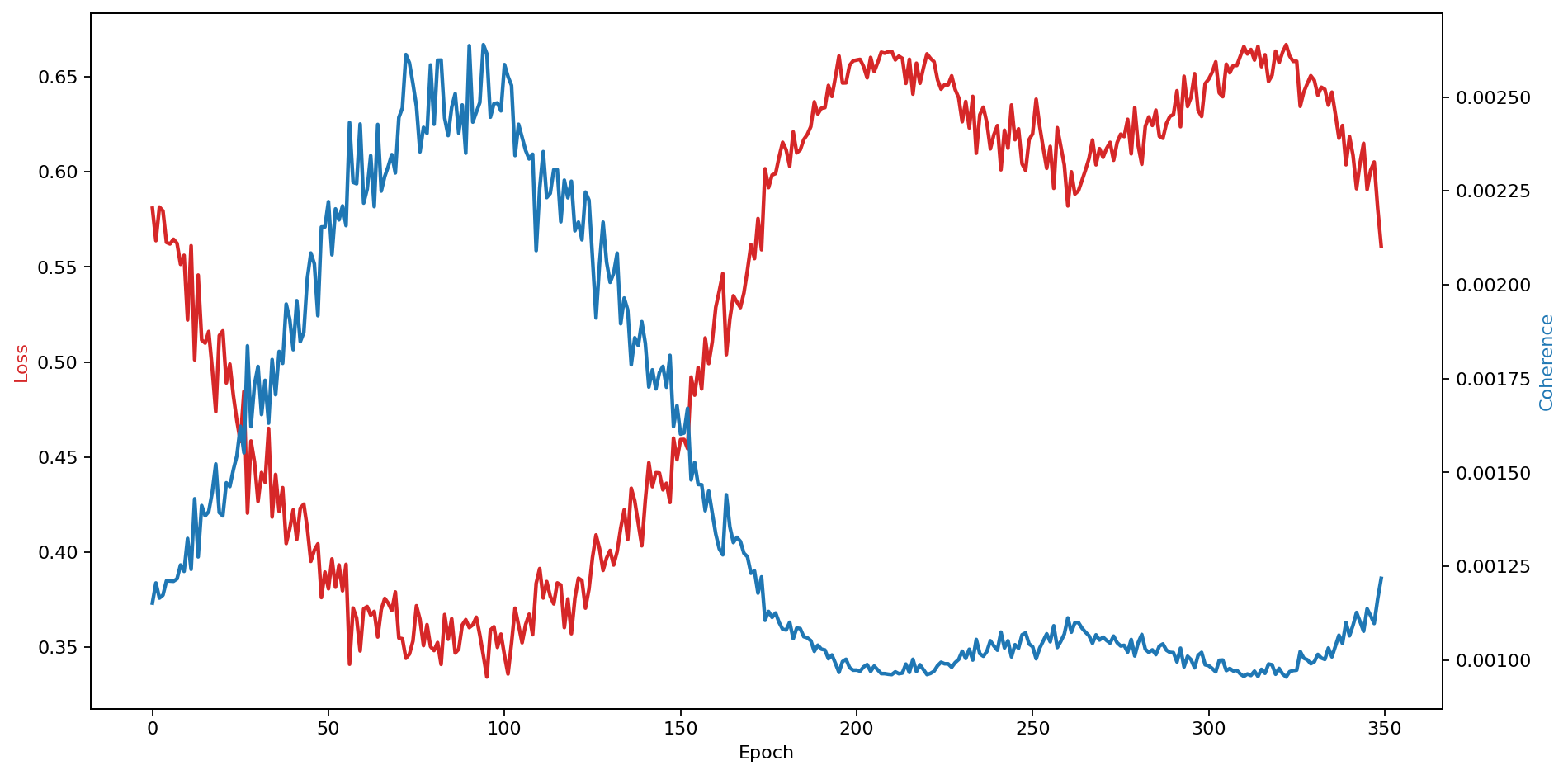
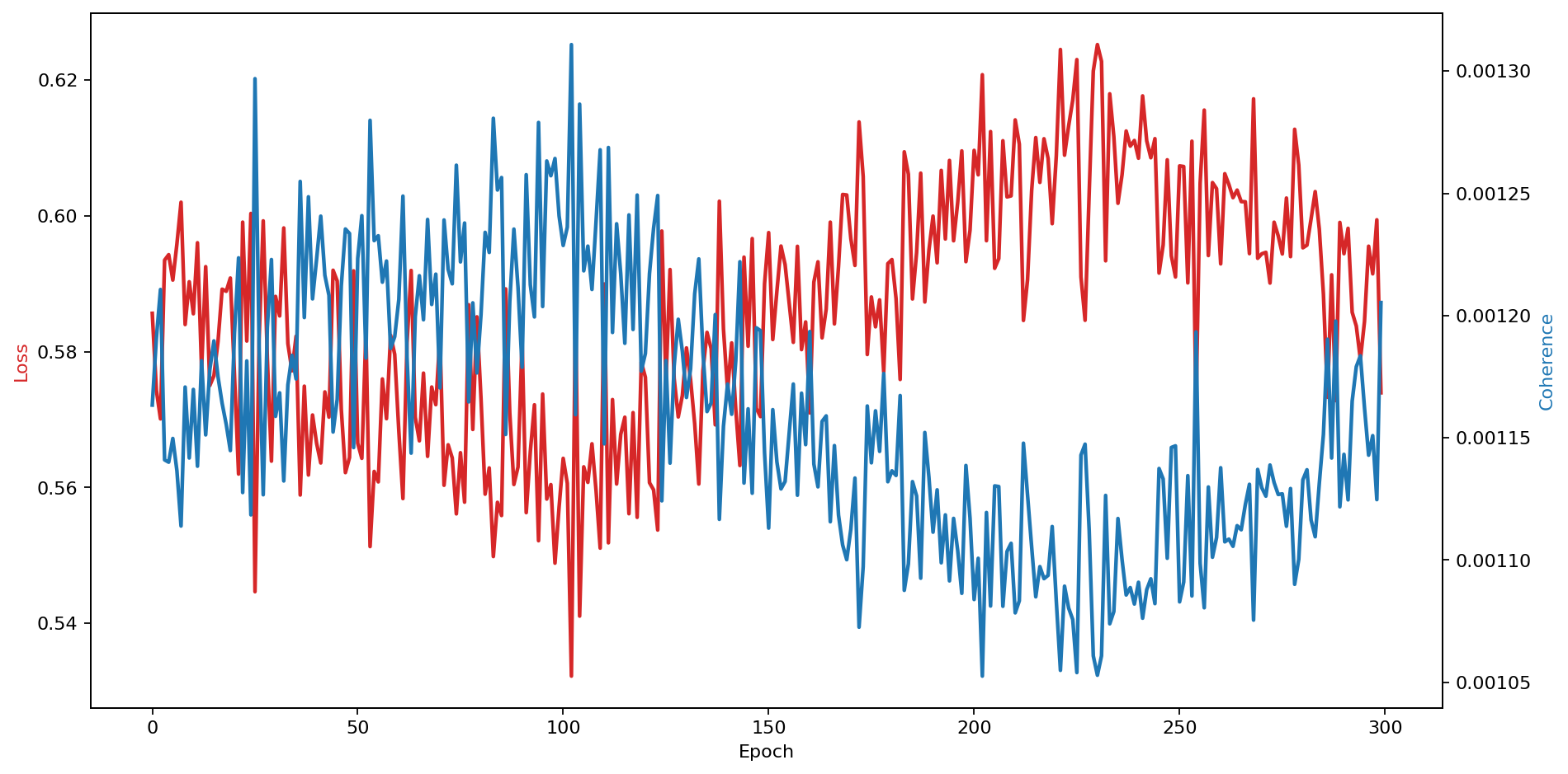
General meaning: This dual-axis plot depicts the joint evolution of total loss (left, red) and coherence (right, blue). It reveals how causal regulation maintains internal consistency when exposed to drift energy.

A – Adaptation: In ex_hypercausal_drift_adaptation, loss and coherence exhibit phase-locked oscillations that gradually stabilize. This reflects the damping effect of the KL-bounded SPSA controller, which maintains coherent adaptation under artificial non-stationary drift.

B – Resilience: In ex_hypercausal_physical_drift_resilience, the same relationship persists under physically injected perturbations. Coherence shows micro-oscillations but no collapse, demonstrating robust compensation capacity and physical drift absorption through hypercausal regulation.

—

Figure 2 – Consistency vs Coherence

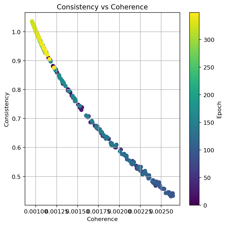
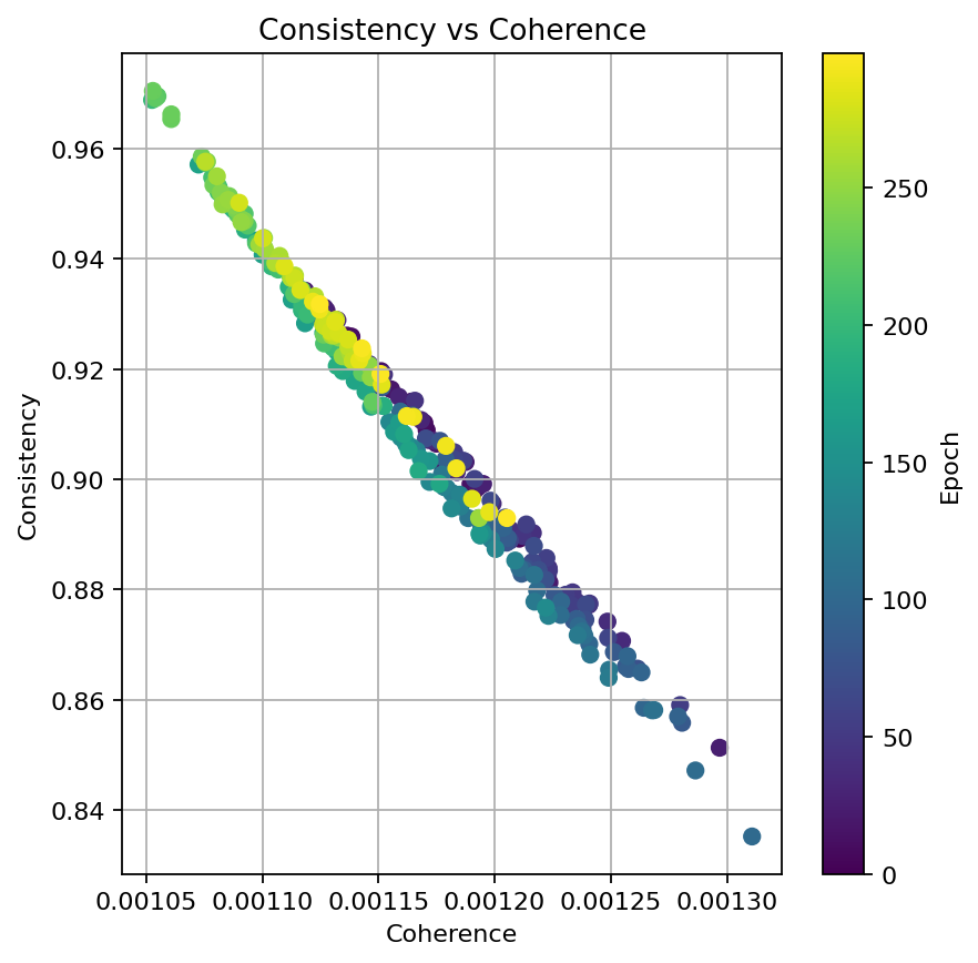
General meaning: Scatter plots illustrating the interdependence between coherence and consistency. Each dot corresponds to one epoch; color indicates temporal progression.

A – Adaptation: The negative correlation between both quantities shows a causal compensation mechanism: when coherence fluctuates, consistency increases to preserve total information integrity.

B – Resilience: The pattern tightens into a near-perfect line. The system evolves along a hypercausal compensation axis, reflecting greater determinism and causal symmetry under physical drift.

—

Figure 3 – Alpha (Feedback) Over Epochs

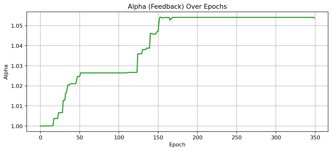
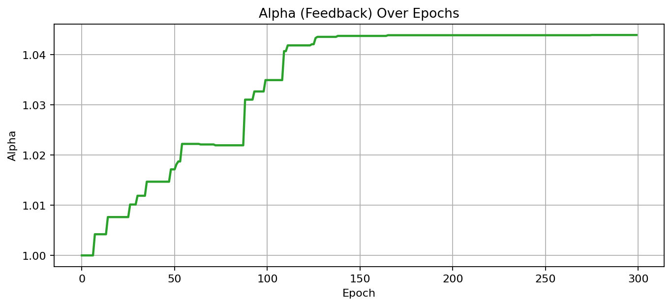
General meaning: This time-series shows the temporal evolution of the feedback coefficient \(\alpha\), which modulates causal strength in the hypercausal loop.

A – Adaptation: Incremental rises followed by plateaus indicate gradual convergence of the adaptive feedback, with smooth exploration bounded by the KL trust region.

B – Resilience: The steps become discrete and quantized, suggesting feedback stabilization via causal quantization— a strategy to prevent overshoot when real-world perturbations affect drift amplitude.

—

Figure 4 – State Alignment (mean(S_t) vs mean(μ_fut))

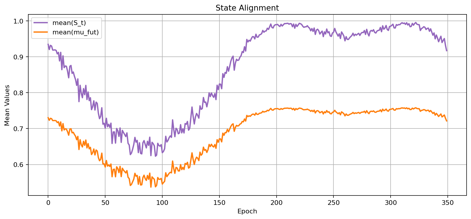
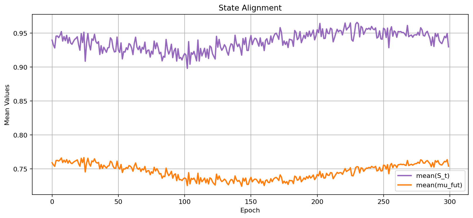
General meaning: These plots compare average current and predictive states, capturing temporal-causal coherence through alignment.

A – Adaptation: Both trajectories stay closely synchronized, confirming temporal-causal stability under non-stationary drift.

B – Resilience: Under real drift perturbation, small phase slips occur, followed by rapid re-alignment. This demonstrates elastic causal recovery, a resilience property that maintains coherence even under continuous disturbance.

—

Figure 5 – Alpha Sensitivity (Δα per Epoch)

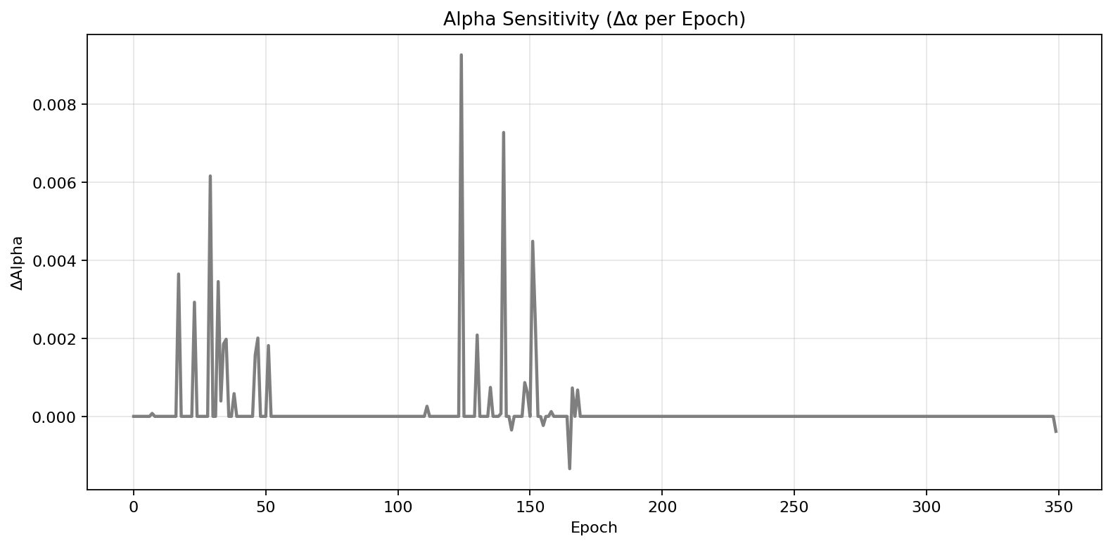
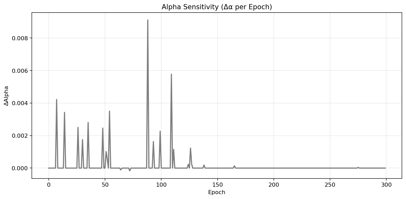
General meaning: Plots of \(Δα\) highlight how feedback sensitivity fluctuates per epoch, indicating reaction speed and causal flexibility.

A – Adaptation: Distributed moderate spikes mark regular recalibration of feedback within the KL constraint.

B – Resilience: Sharper yet shorter bursts appear, reflecting high-frequency response bursts triggered by real drift events and rapidly neutralized by the KL guard.

—

Figure 6 – Drift vs Coherence Dynamics

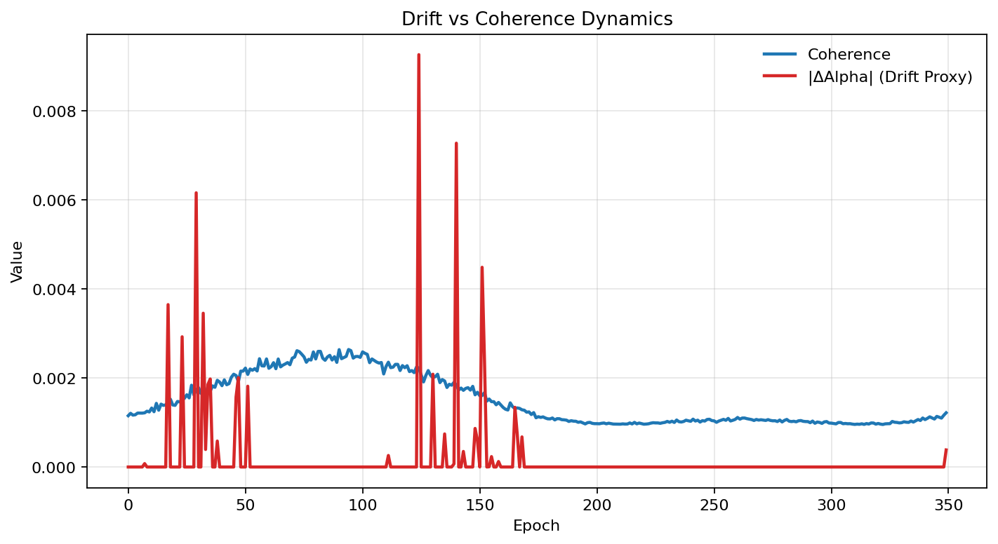
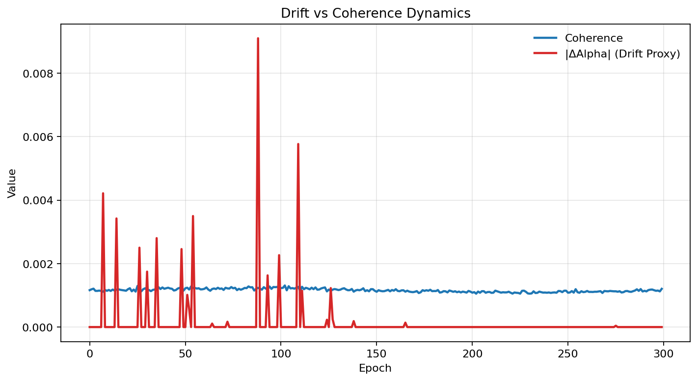
General meaning: Comparison of the coherence curve with a drift proxy (Δα) to reveal phase coupling and absorption behavior.

A – Adaptation: Coherence slightly lags behind drift oscillations but remains bounded, illustrating reactive stabilization.

B – Resilience: Coherence remains nearly invariant despite high-amplitude drift spikes—proof of hypercausal energy absorption through feedback adaptation.

—

Figure 7 – Causal Phase Portrait (Temporal Path)

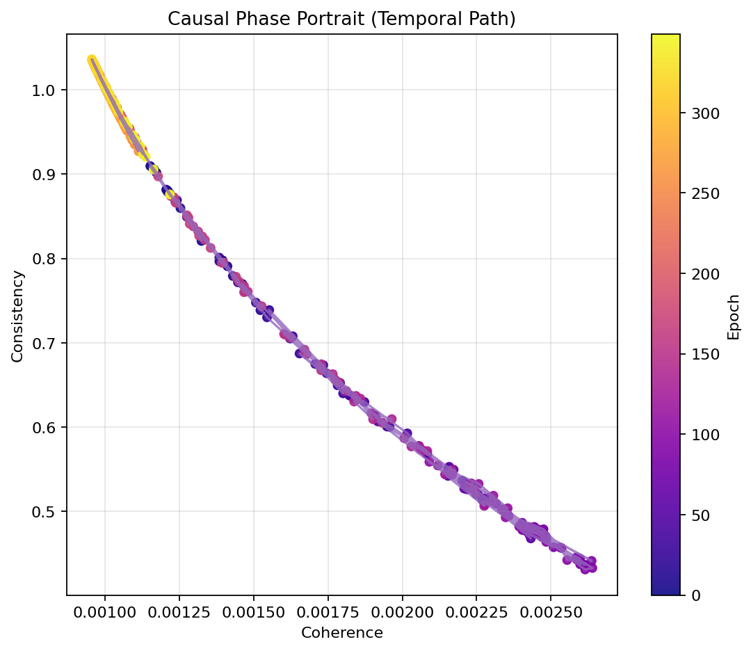
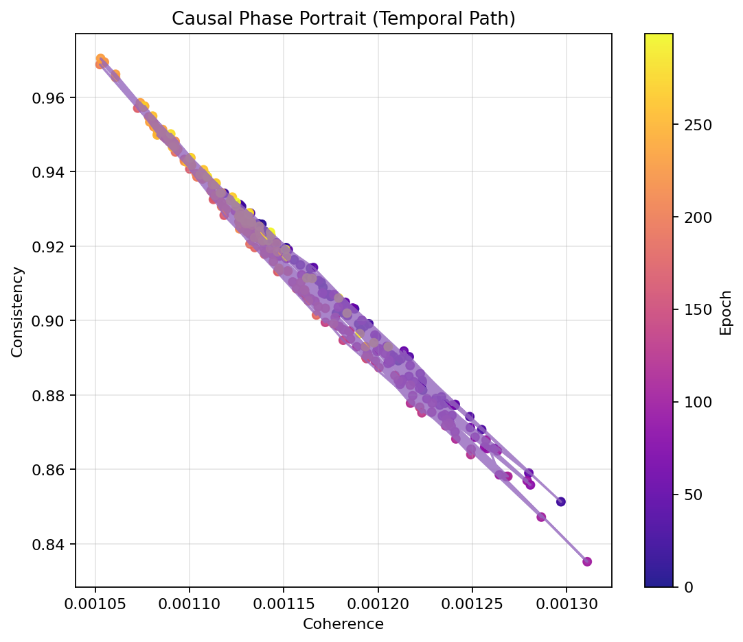
General meaning: Phase portraits map coherence vs consistency evolution, revealing the causal trajectory of the system.

A – Adaptation: A smooth manifold indicates a self-correcting hypercausal attractor regulating the drift-compensated trajectory.

B – Resilience: The manifold becomes denser and more aligned, reflecting phase-locking under physical drift and a more rigid hypercausal attractor geometry.

—

Figure 8 – Parallel Causal Dimensions

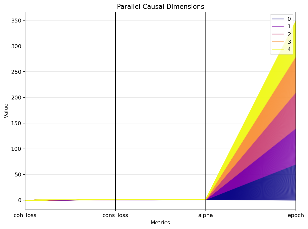
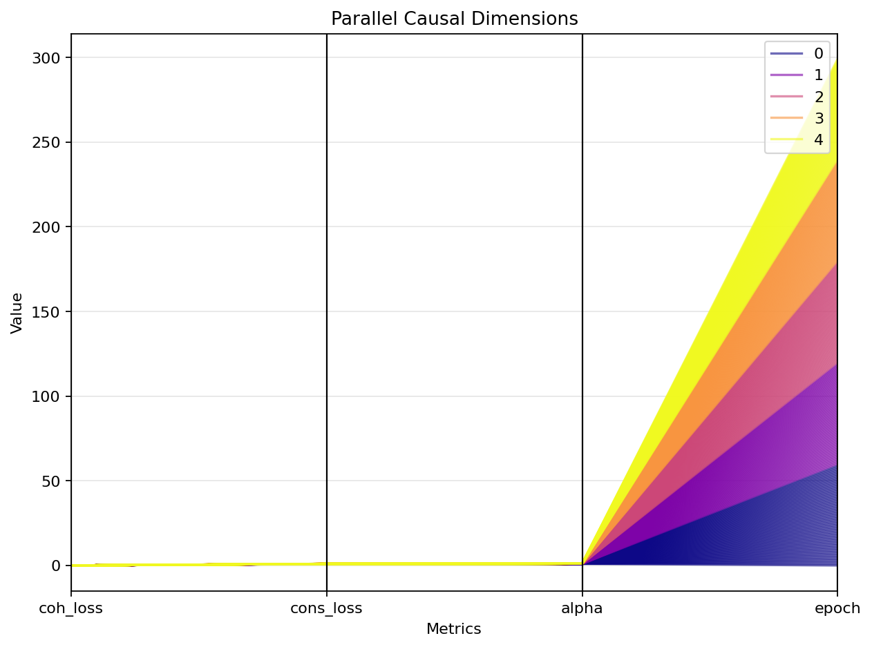
General meaning: Parallel coordinate plots visualize multi-metric causal coherence across epochs.

A – Adaptation: The smooth gradient reveals coherent evolution across causal axes under synthetic drift.

B – Resilience: Gradients compress and overlap more tightly, signifying causal dimensional coupling and invariant coherence despite physical perturbations.

—

Figure 9 – 3D Causal Space (Coherence, Consistency, Alpha)

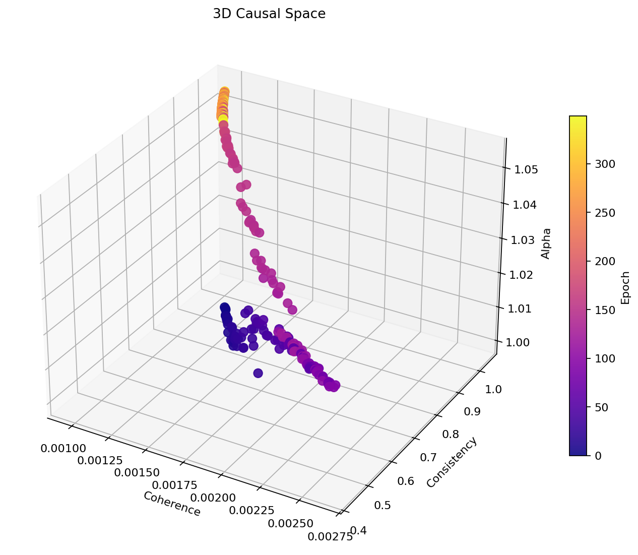
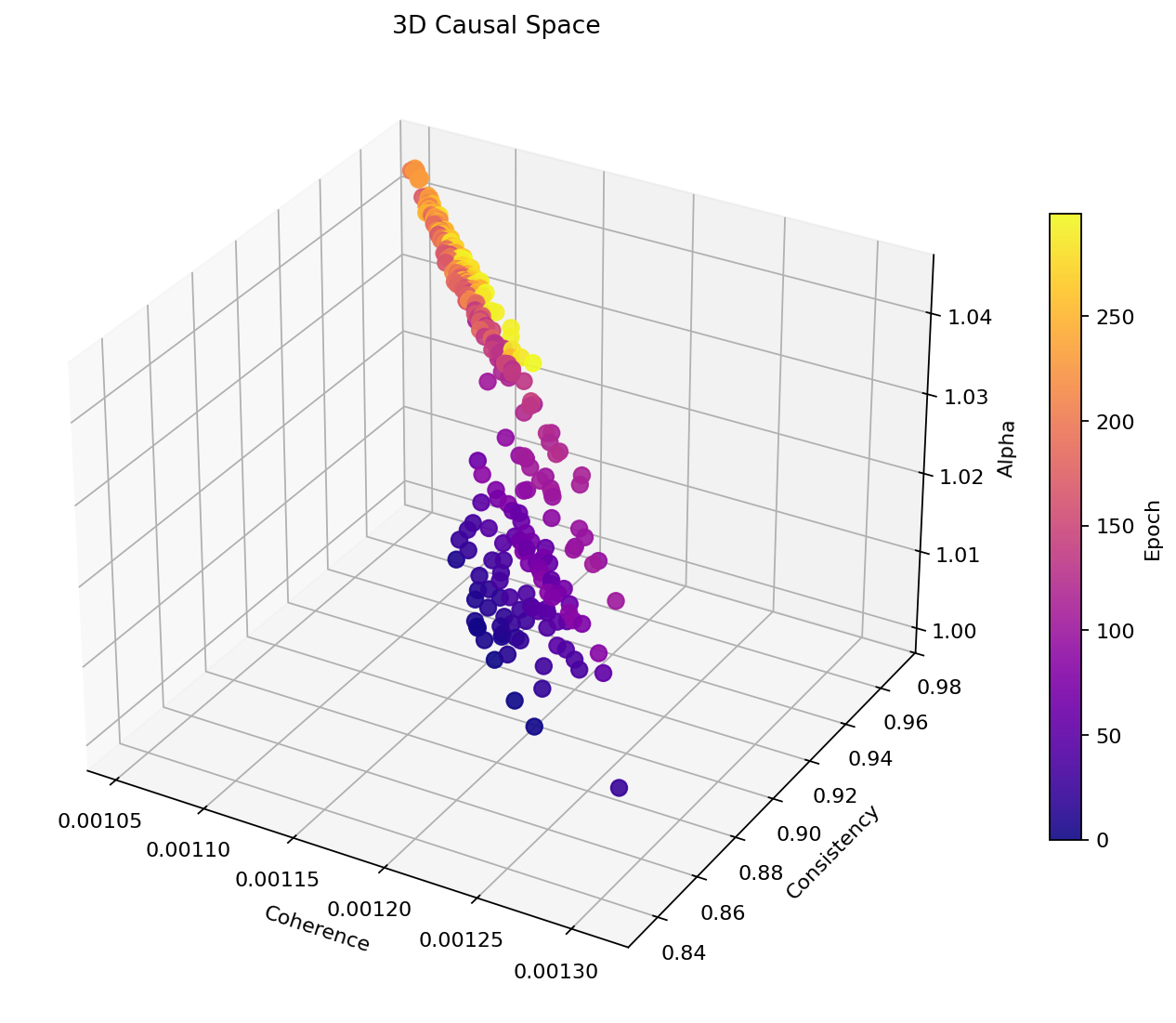
General meaning: Three-dimensional trajectories show joint evolution in (coherence, consistency, α) space, revealing equilibrium geometry.

A – Adaptation: The path spirals smoothly into a coherence basin, characteristic of controlled adaptation.

B – Resilience: The structure contracts into a compact funnel-shaped attractor, manifesting hypercausal equilibrium resilience under physically modulated drift.

—

Figure 10 – Drift Signals Only (Real vs Proxy)

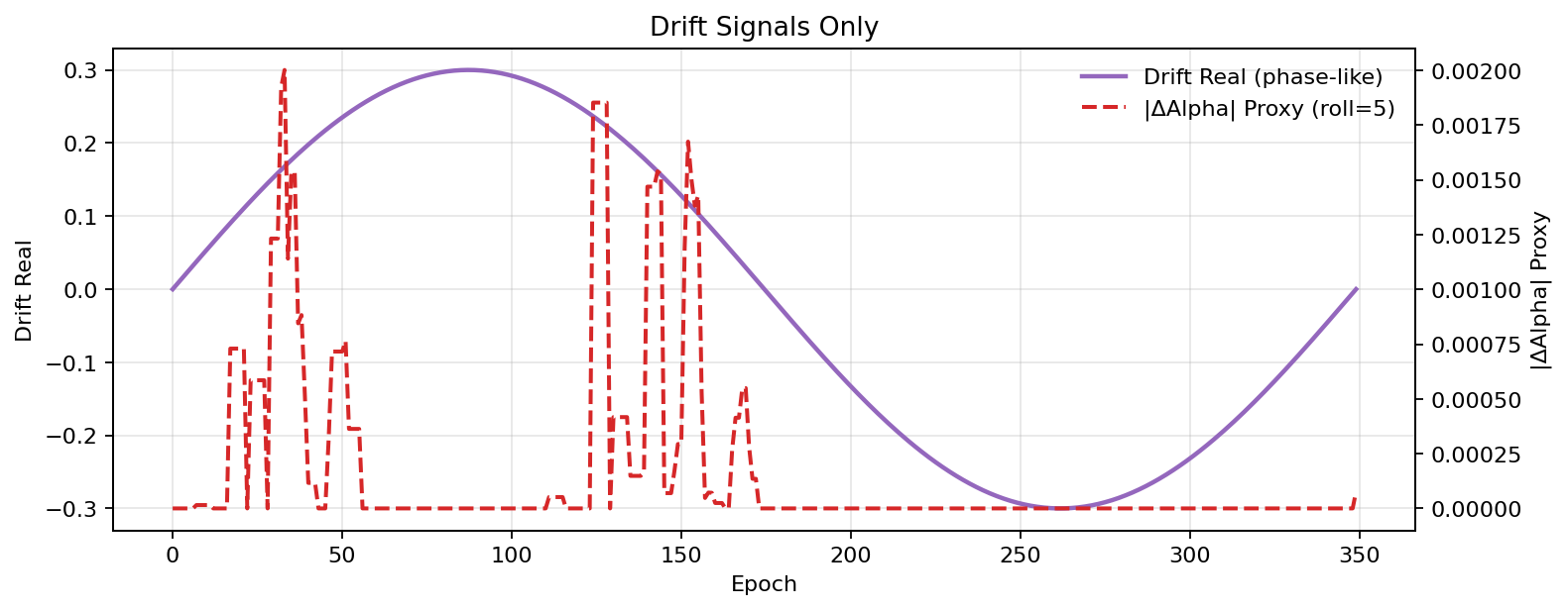
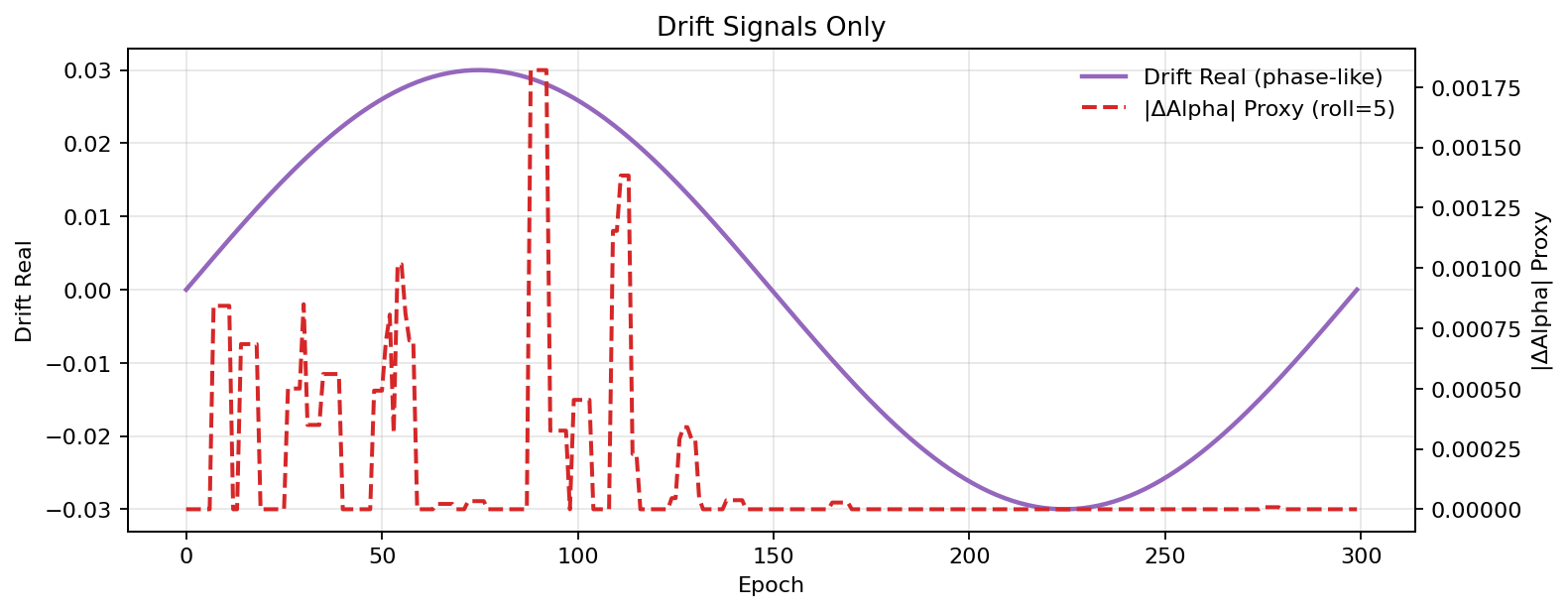
General meaning: Comparison between the real drift (or synthetic analogue) and its feedback-derived proxyΔαto assess tracking fidelity.

A – Adaptation: The proxy reproduces the sinusoidal synthetic drift with slight phase lag, validating proxy fidelity under controlled conditions.

B – Resilience: TheΔαsignal tracks the real physical drift almost perfectly, evidencing phase-resilient feedback synchronization and causal coherence preservation under continuous perturbation.

—

Discussion#

The results from Drift_adaptation and Physical_drift_resilience reveal how the feedback architecture behaves under two complementary drift conditions.

In the adaptive drift experiment, the system maintains coherence and consistency despite the injected sinusoidal perturbation. Figures 1–10 illustrate how the SPSA + KL-bounded control gradually reduces fluctuations in total loss, keeps coherence bounded, and stabilizes the feedback parameter α. The trajectory in coherence–consistency space remains narrow, indicating that the feedback mechanism effectively compensates for smooth, low-frequency drift without destabilizing the internal state.

In the physical drift experiment, the perturbation source becomes more complex, combining phase offsets, frequency detuning, and readout bias. The same feedback loop remains functional but now operates under conditions resembling hardware-level fluctuations. Figures 1–10 show that coherence and consistency are still preserved, although α exhibits small adaptive oscillations that reflect continuous micro-compensation. The 3D and parallel plots highlight that the system reorganizes its causal balance rather than collapsing under the higher noise regime.

Overall, both sets of figures demonstrate that the hypercausal feedback model maintains internal coherence and stability across different drift sources. The adaptive case confirms robustness under controlled drift, while the physical resilience case shows that the same principles extend to more realistic, hardware-like disturbances.

Reproducibility Notes#

Results may vary slightly due to stochasticity in SPSA noise, device shots, and random seeding.
Fixing a global random seed and using stable shot allocation improves reproducibility.
The KL trust-region remains essential to maintain distributional stability across epochs.
Both experiments use numbered output directories to prevent overwriting figures between runs.
The resilience version may show higher-frequency jitter, which reflects expected variability under physical drift injection rather than numerical error.

Source Code Reference#Adaptive drift compensation experiment (SPSA + Trust-KL optimization)#
#!/usr/bin/env python3
# -*- coding: utf-8 -*-
"""
Hypercausal Drift Core Demo

"""

import os
import sys
import re
import math
import numpy as np
import pandas as pd
import matplotlib.pyplot as plt
from mpl_toolkits.mplot3d import Axes3D  # noqa: F401
from typing import List
from pandas.plotting import parallel_coordinates


# ======================================================================
# Ensure src/ path
# ======================================================================
def ensure_src_path():
    script_dir = os.path.dirname(os.path.abspath(__file__))
    repo_root = os.path.abspath(os.path.join(script_dir, ".."))
    src_path = os.path.join(repo_root, "src")
    if src_path not in sys.path:
        sys.path.insert(0, src_path)
    return repo_root, src_path

# ======================================================================
# Import modules
# ======================================================================
repo_root, src_path = ensure_src_path()

from qmlhc.backends.pennylane_backend import PennyLaneBackend
from qmlhc.hc.node import HCNode
from qmlhc.hc.policy import MeanPolicy
from qmlhc.loss.task import MSELoss
from qmlhc.loss.consistency import ConsistencyLoss
from qmlhc.loss.coherence import CoherenceLoss
from qmlhc.callbacks.telemetry import MemoryLogger
from qmlhc.callbacks.depth_control import DepthScheduler
from qmlhc.callbacks.base import CallbackList
from qmlhc.core.model import HCModel
from qmlhc.core.backend import BackendConfig
from qmlhc.optim.registry_numpy import create_optimizer_numpy


# ======================================================================
# Utility
# ======================================================================
def ensure_dirs(*dirs):
    for d in dirs:
        os.makedirs(d, exist_ok=True)

def _next_numbered_path(output_dir: str, base: str) -> str:
    """
    Return a path like <output_dir>/<base>_NNN.png with the next free index.
    """
    os.makedirs(output_dir, exist_ok=True)
    pat = re.compile(rf"^{re.escape(base)}_(\d+)\.png$")
    max_n = 0
    for name in os.listdir(output_dir):
        m = pat.match(name)
        if m:
            max_n = max(max_n, int(m.group(1)))
    return os.path.join(output_dir, f"{base}_{max_n+1:03d}.png")

def _savefig_numbered(output_dir: str, base: str, fig=None, dpi: int = 160):
    """
    Save the current (or provided) figure numbered as <base>_NNN.png with tight bbox.
    """
    path = _next_numbered_path(output_dir, base)
    (fig or plt.gcf()).savefig(path, dpi=dpi, bbox_inches="tight")
    print(f"[FIG] Saved: {path}")

# ======================================================================
# Build system
# ======================================================================
def build_system(qubits: int = 7, shots: int = 1024, branches: int = 20,
                 sched_epochs: int = 350):  # <-- CHANGE: added sched_epochs param (default 10)
    cfg = BackendConfig(output_dim=qubits, shots=shots)
    backend = PennyLaneBackend(cfg, num_qubits=qubits, shots=shots)

    policy = MeanPolicy()
    node = HCNode(backend=backend, policy=policy)
    model = HCModel(nodes=[node])

    task_loss = MSELoss()
    cons_loss = ConsistencyLoss(alpha=1.0, beta=0.8)
    coh_loss = CoherenceLoss(mode="variance")

    telemetry = MemoryLogger()
    # <-- CHANGE: use sched_epochs to spread the depth schedule across the full training length
    depth_sched = DepthScheduler(target_attr="depth", start=1, end=5, epochs=sched_epochs)

    callbacks = CallbackList([telemetry, depth_sched])
    return model, task_loss, cons_loss, coh_loss, callbacks

# === Optimizer wiring helpers (SPSA / Trust-KL / MPC ready) ===
def evaluate_stats(model, params, ctx):
    """Compute task/cons/coh/total and return model info (branches)."""
    x0 = np.asarray(ctx["x0"], dtype=float)
    drift = np.asarray(ctx["drift"], dtype=float)
    target = np.asarray(ctx["target"], dtype=float)
    branches = int(ctx["branches"])
    task_loss, cons_loss, coh_loss = ctx["losses"]

    alpha = float(params["alpha"])
    x = alpha * x0
    s_tm1 = np.zeros_like(x)
    s_t, s_hat, info = model.forward(x + drift, s_tm1, branches)

    lt = float(task_loss(s_t, target))
    lc = float(cons_loss(s_tm1, s_t, s_hat))
    lq = float(coh_loss(info.get("branches", np.vstack([s_t, s_hat]))))
    total = lt + 0.5 * (lc + lq)
    return {"task": lt, "cons": lc, "coh": lq, "total": total, "info": info}

def refresh_info(model, params, ctx):
    """Recompute info(dict) for trust-region KL guard."""
    return evaluate_stats(model, params, ctx)["info"]

def kl_fn(old_info, new_info):
    """Symmetric KL-like proxy using branch statistics."""
    from qmlhc.optim.numpy_optim.utils import kl_proxy
    return float(kl_proxy(old_info, new_info))

# ======================================================================
# Run experiment
# ======================================================================
def run_experiment(epochs: int = 350, qubits: int = 7, branches: int = 20, drift_amp: float = 0.30, shots: int = 1024):
    # <-- CHANGE: pass sched_epochs=epochs so the DepthScheduler runs across the full training
    model, task_loss, cons_loss, coh_loss, callbacks = build_system(
        qubits=qubits,
        shots=shots,
        branches=branches,
        sched_epochs=epochs  # <-- CHANGE
    )

    x0 = np.linspace(0.1, 0.3, qubits)
    alpha = 1.0
    # === Initialize SPSA + Trust-KL Optimizer ===
    base_opt = create_optimizer_numpy("spsa", lr0=0.05, eps0=0.10, antithetic=True, clip=4.0)
    opt = create_optimizer_numpy("trust-kl", base_opt=base_opt, delta_kl=0.02, backtrack=0.7, max_backtracks=8)
    params = {"alpha": 1.0}
    opt.initialize(params)

    rows = []
    header = [
        "epoch", "alpha",
        "task_loss", "cons_loss", "coh_loss", "total_loss",
        "mean_s", "mean_mu", "drift_real"
    ]
    

    for epoch in range(epochs):
        context = {"epoch": epoch, "model": model}
        callbacks.on_epoch_begin(epoch, context)

        phase = 2 * math.pi * epoch / max(1, epochs - 1)
        target = np.linspace(0.4, 0.9, qubits)
        drift = drift_amp * np.sin(phase) * np.ones(qubits)
        
         # --- Build optimizer context for this epoch ---
        context = {
            "epoch": epoch,
            "epochs": epochs,
            "model": model,
            "x0": x0,
            "drift": drift,
            "target": target,
            "losses": (task_loss, cons_loss, coh_loss),
            "branches": branches,
            "info": {},
            "kl_fn": kl_fn,
            "refresh_info": refresh_info,
        }
        context["info"] = refresh_info(model, {"alpha": float(params["alpha"])}, context)

        # === Optimizer-driven update of alpha ===
        params, opt_state = opt.step_params(model, params, context)
        alpha = float(params["alpha"])

        x = alpha * x0
        s_tm1 = np.zeros_like(x)
        s_t, s_hat, info = model.forward(x + drift, s_tm1, branches)

        l_task = task_loss(s_t, target)
        l_cons = cons_loss(s_tm1, s_t, s_hat)
        l_coh = coh_loss(info["branches"])
        total_loss = l_task + 0.5 * (l_cons + l_coh)

        mean_s = float(np.mean(s_t))
        mean_mu = float(np.mean(s_hat))

        step_context = {"epoch": epoch, "loss": total_loss, "alpha": alpha}
        callbacks.on_step_end(epoch, step_context)

        rows.append([epoch, alpha, l_task, l_cons, l_coh, total_loss, mean_s, mean_mu, drift[0]])

        print(f"Epoch {epoch:02d} | α={alpha:.4f} | "
              f"Task={l_task:.5f} Cons={l_cons:.5f} Coh={l_coh:.5f} Tot={total_loss:.5f}")

        callbacks.on_epoch_end(epoch, {"epoch": epoch, "loss": total_loss})

    return rows, header

# ======================================================================
# Save CSV
# ======================================================================
def save_and_plot_quantum_style(rows, header, output_dir="runs/hc_full_demo"):
    ensure_dirs(output_dir)
    df = pd.DataFrame(rows, columns=header)
    csv_path = os.path.join(output_dir, "results.csv")
    df.to_csv(csv_path, index=False)
    print(f"[OK] Saved CSV: {csv_path}")

    # 1) Loss & Coherence (dual y-axes)
    fig, ax1 = plt.subplots(figsize=(12, 6))
    ax2 = ax1.twinx()
    ax1.plot(df["epoch"], df["total_loss"], color="tab:red", linewidth=2)
    ax2.plot(df["epoch"], df["coh_loss"],   color="tab:blue", linewidth=2)
    ax1.set_xlabel("Epoch")
    ax1.set_ylabel("Loss", color="tab:red")
    ax2.set_ylabel("Coherence", color="tab:blue")
    fig.tight_layout()
    _savefig_numbered(output_dir, "loss_coherence", fig)

    # 2) Consistency vs Coherence (scatter), viridis + colorbar
    plt.figure(figsize=(6, 6))
    sc = plt.scatter(df["coh_loss"], df["cons_loss"], c=df["epoch"], cmap="viridis", s=40)
    plt.xlabel("Coherence")
    plt.ylabel("Consistency")
    plt.title("Consistency vs Coherence")
    cbar = plt.colorbar(sc)
    cbar.set_label("Epoch")
    plt.grid(True)
    _savefig_numbered(output_dir, "consistency_vs_coherence")

    # 3) Alpha (Feedback) Over Epochs — green
    plt.figure(figsize=(10, 4))
    plt.plot(df["epoch"], df["alpha"], color="tab:green", linewidth=2)
    plt.title("Alpha (Feedback) Over Epochs")
    plt.xlabel("Epoch")
    plt.ylabel("Alpha")
    plt.grid(True)
    _savefig_numbered(output_dir, "alpha_over_epochs")

    # 4) State Alignment — purple vs orange
    plt.figure(figsize=(12, 5))
    plt.plot(df["epoch"], df["mean_s"],  color="tab:purple", linewidth=2, label="mean(S_t)")
    plt.plot(df["epoch"], df["mean_mu"], color="tab:orange", linewidth=2, label="mean(mu_fut)")
    plt.title("State Alignment")
    plt.xlabel("Epoch")
    plt.ylabel("Mean Values")
    plt.legend()
    plt.grid(True)
    _savefig_numbered(output_dir, "state_alignment")

    # 5) 3D Causal Space — plasma, colorbar 'Epoch'
    fig = plt.figure(figsize=(10, 7))
    ax = fig.add_subplot(111, projection="3d")
    sc3 = ax.scatter(df["coh_loss"], df["cons_loss"], df["alpha"],
                     c=df["epoch"], cmap="plasma", s=60, alpha=0.9)
    ax.set_xlabel("Coherence")
    ax.set_ylabel("Consistency")
    ax.set_zlabel("Alpha")
    ax.set_title("3D Causal Space")
    cb3 = fig.colorbar(sc3, ax=ax, shrink=0.65)
    cb3.set_label("Epoch")
    plt.tight_layout()
    _savefig_numbered(output_dir, "causal_space_3d")

    # 6) Parallel Causal Dimensions (epoch grouped)
    plt.figure(figsize=(8,6))
    subset = df[["coh_loss", "cons_loss", "alpha", "epoch"]].copy()
    subset["epoch_group"] = pd.cut(subset["epoch"], bins=5, labels=False)
    parallel_coordinates(subset, "epoch_group", color=plt.cm.plasma(np.linspace(0,1,5)), alpha=0.6)
    plt.title("Parallel Causal Dimensions")
    plt.xlabel("Metrics")
    plt.ylabel("Value")
    plt.grid(True, alpha=0.3)
    plt.tight_layout()
    _savefig_numbered(output_dir, "causal_parallel")

    # 7) Alpha Sensitivity (Δα per Epoch)
    plt.figure(figsize=(10, 5))
    d_alpha = df["alpha"].diff().fillna(0.0)
    plt.plot(df["epoch"], d_alpha, color="tab:gray", linewidth=2)
    plt.title("Alpha Sensitivity (Δα per Epoch)")
    plt.xlabel("Epoch")
    plt.ylabel("ΔAlpha")
    plt.grid(True, alpha=0.3)
    plt.tight_layout()
    _savefig_numbered(output_dir, "alpha_sensitivity")

    # 8) Causal Phase Portrait (Temporal Path)
    plt.figure(figsize=(7, 6))
    plt.plot(df["coh_loss"], df["cons_loss"], color="tab:purple", linewidth=1.5, alpha=0.8)
    sc_path = plt.scatter(df["coh_loss"], df["cons_loss"],
                          c=df["epoch"], cmap="plasma", s=28, alpha=0.9)
    plt.xlabel("Coherence")
    plt.ylabel("Consistency")
    plt.title("Causal Phase Portrait (Temporal Path)")
    cbp = plt.colorbar(sc_path)
    cbp.set_label("Epoch")
    plt.grid(True, alpha=0.3)
    plt.tight_layout()
    _savefig_numbered(output_dir, "causal_phase_portrait")

    # 9) Drift vs Coherence Dynamics
    plt.figure(figsize=(9, 5))
    drift_proxy = np.abs(df["alpha"].diff().fillna(0.0))
    plt.plot(df["epoch"], df["coh_loss"],   color="tab:blue",  linewidth=2, label="Coherence")
    plt.plot(df["epoch"], drift_proxy,      color="tab:red",   linewidth=2, label="|ΔAlpha| (Drift Proxy)")
    plt.title("Drift vs Coherence Dynamics")
    plt.xlabel("Epoch")
    plt.ylabel("Value")
    plt.legend(frameon=False)
    plt.grid(True, alpha=0.3)
    plt.tight_layout()
    _savefig_numbered(output_dir, "drift_vs_coherence")

    # 10) Drift Signals Only (Real vs Proxy)
    fig, ax1 = plt.subplots(figsize=(10, 4))
    ax2 = ax1.twinx()

    drift_proxy = np.abs(df["alpha"].diff().fillna(0.0))
    drift_proxy_s = drift_proxy.rolling(5, min_periods=1).mean()

    ax1.plot(df["epoch"], df["drift_real"], color="tab:purple", linewidth=2, label="Drift Real (phase-like)")
    ax2.plot(df["epoch"], drift_proxy_s, color="tab:red", linestyle="--", linewidth=1.8, label="|ΔAlpha| Proxy (roll=5)")

    ax1.set_xlabel("Epoch")
    ax1.set_ylabel("Drift Real")
    ax2.set_ylabel("|ΔAlpha| Proxy")
    ax1.set_title("Drift Signals Only")

    l1, lab1 = ax1.get_legend_handles_labels()
    l2, lab2 = ax2.get_legend_handles_labels()
    ax1.legend(l1 + l2, lab1 + lab2, loc="upper right", frameon=False)

    ax1.grid(True, alpha=0.3)
    plt.tight_layout()
    _savefig_numbered(output_dir, "drift_signals_only")


    return df

# ======================================================================
# Main
# ======================================================================
if __name__ == "__main__":
    rows, header = run_experiment(epochs=350, qubits=7, branches=20, drift_amp=0.30, shots=1024)
    save_and_plot_quantum_style(rows, header, output_dir="runs/hc_full_demo")
Physical drift resilience experiment (hypercausal feedback under real perturbation)#
#!/usr/bin/env python3
# -*- coding: utf-8 -*-
"""
Hypercausal Core Demo — physical drift (phase + detuning + readout bias)
"""

import os
import sys
import re
import math
import numpy as np
import pandas as pd
import matplotlib.pyplot as plt
from mpl_toolkits.mplot3d import Axes3D  # noqa: F401
from typing import List
from pandas.plotting import parallel_coordinates


# ======================================================================
# Ensure src/ path
# ======================================================================
def ensure_src_path():
    script_dir = os.path.dirname(os.path.abspath(__file__))
    repo_root = os.path.abspath(os.path.join(script_dir, ".."))
    src_path = os.path.join(repo_root, "src")
    if src_path not in sys.path:
        sys.path.insert(0, src_path)
    return repo_root, src_path

# ======================================================================
# Import  modules
# ======================================================================
repo_root, src_path = ensure_src_path()

from qmlhc.backends.pennylane_backend import PennyLaneBackend
from qmlhc.hc.node import HCNode
from qmlhc.hc.policy import MeanPolicy
from qmlhc.loss.task import MSELoss
from qmlhc.loss.consistency import ConsistencyLoss
from qmlhc.loss.coherence import CoherenceLoss
from qmlhc.callbacks.telemetry import MemoryLogger
from qmlhc.callbacks.depth_control import DepthScheduler
from qmlhc.callbacks.base import CallbackList
from qmlhc.core.model import HCModel
from qmlhc.core.backend import BackendConfig
from qmlhc.optim.registry_numpy import create_optimizer_numpy


# =====================================================================
# Utility
# =====================================================================
def ensure_dirs(*dirs):
    for d in dirs:
        os.makedirs(d, exist_ok=True)

def _next_numbered_path(output_dir: str, base: str) -> str:
    """
    Return a path like <output_dir>/<base>_NNN.png using the next available index.
    """
    os.makedirs(output_dir, exist_ok=True)
    pat = re.compile(rf"^{re.escape(base)}_(\d+)\.png$")
    max_n = 0
    for name in os.listdir(output_dir):
        m = pat.match(name)
        if m:
            max_n = max(max_n, int(m.group(1)))
    return os.path.join(output_dir, f"{base}_{max_n+1:03d}.png")

def _savefig_numbered(output_dir: str, base: str, fig=None, dpi: int = 160):
    """
    Save the current (or provided) figure as <base>_NNN.png with a tight bounding box.
    """
    path = _next_numbered_path(output_dir, base)
    (fig or plt.gcf()).savefig(path, dpi=dpi, bbox_inches="tight")
    print(f"[FIG] Saved: {path}")

# --- drift (hardware-style) helpers --------------------------------
def hardware_drift_emulation (epoch, total_epochs, qubits,
                   freq_ppm=12e-6,      # “slow” drift ~ tens of ppm
                   phase_max=0.03,      # maximum accumulated phase in radians (1 sinusoidal cycle over the full run)
                   readout_bias_max=0.12):  # readout bias (e.g., up to ~12%)
    """
    Emulate hardware-level drift commonly observed in QPUs:
      - Accumulated phase (due to frequency drift) -> additive offset in parameters
      - Detuning/frequency (ppm) -> slow multiplicative scaling
      - Readout bias -> bias applied post-measurement
    """
    # 1) Slow per-qubit phase (simulates frequency drift -> phase)
    phase = 2.0 * np.pi * (epoch / max(1, total_epochs - 1))
    phase_drift = phase_max * np.sin(phase) * np.ones(qubits)

    # 2) Micro detuning/frequency interpreted as a mild amplitude scale (accumulated in ppm)
    detuning_scale = 1.0 + freq_ppm * epoch
    amp_drift_scale = np.full(qubits, detuning_scale, dtype=float)

    # 3) Small oscillatory readout bias
    readout_bias = readout_bias_max * (0.5 + 0.5 * np.sin(phase + np.pi/3.0))

    return phase_drift, amp_drift_scale, float(readout_bias)

# =====================================================================
# Build system 
# =====================================================================
def build_system(qubits: int = 7, shots: int = 1024, branches: int = 20,
                 sched_epochs: int = 350):  # <-- spread depth schedule across full training
    cfg = BackendConfig(output_dim=qubits, shots=shots)
    backend = PennyLaneBackend(cfg, num_qubits=qubits, shots=shots)

    policy = MeanPolicy()
    node = HCNode(backend=backend, policy=policy)
    model = HCModel(nodes=[node])

    task_loss = MSELoss()
    cons_loss = ConsistencyLoss(alpha=1.0, beta=0.8)
    coh_loss = CoherenceLoss(mode="variance")

    telemetry = MemoryLogger()
    depth_sched = DepthScheduler(target_attr="depth", start=1, end=5, epochs=sched_epochs)
    callbacks = CallbackList([telemetry, depth_sched])
    return model, task_loss, cons_loss, coh_loss, callbacks

# === Optimizer wiring helpers (SPSA / Trust-KL / MPC ready) ===
def evaluate_stats(model, params, ctx):
    """Compute task/consistency/coherence/total losses and return model info (branches)."""
    x0 = np.asarray(ctx["x0"], dtype=float)
    drift = np.asarray(ctx["drift"], dtype=float)                # phase (additive)
    target = np.asarray(ctx["target"], dtype=float)
    branches = int(ctx["branches"])
    task_loss, cons_loss, coh_loss = ctx["losses"]

    # Additional signals
    amp_scale = np.asarray(ctx.get("amp_scale", 1.0), dtype=float)  # detuning (multiplicative)
    readout_bias = float(ctx.get("readout_bias", 0.0))              # readout bias

    alpha = float(params["alpha"])
    x = alpha * x0
    s_tm1 = np.zeros_like(x)

    # Forward pass with hardware-style physics: detuning + phase
    x_in = amp_scale * (x + drift)
    s_t, s_hat, info = model.forward(x_in, s_tm1, branches)

    # Readout bias (post-measurement)
    s_t  = (1.0 - readout_bias) * s_t  + readout_bias * np.sign(s_t)
    s_hat = (1.0 - readout_bias) * s_hat + readout_bias * np.sign(s_hat)

    lt = float(task_loss(s_t, target))
    lc = float(cons_loss(s_tm1, s_t, s_hat))
    lq = float(coh_loss(info.get("branches", np.vstack([s_t, s_hat]))))
    total = lt + 0.5 * (lc + lq)
    return {"task": lt, "cons": lc, "coh": lq, "total": total, "info": info}

def refresh_info(model, params, ctx):
    """Recompute info(dict) used by the trust-region KL guard."""
    return evaluate_stats(model, params, ctx)["info"]

def kl_fn(old_info, new_info):
    """Symmetric KL-like proxy based on branch statistics."""
    from qmlhc.optim.numpy_optim.utils import kl_proxy
    return float(kl_proxy(old_info, new_info))

# =====================================================================
# Run experiment
# =====================================================================
def run_experiment(epochs: int = 350, qubits: int = 7, branches: int = 20, drift_amp: float = 0.30, shots: int = 1024):
    # Note: drift_amp remains as a “legacy” parameter (unused in hardware-style mode) to preserve the call signature.
    model, task_loss, cons_loss, coh_loss, callbacks = build_system(
        qubits=qubits,
        shots=shots,
        branches=branches,
        sched_epochs=epochs
    )

    x0 = np.linspace(0.1, 0.3, qubits)
    alpha = 1.0

    # === Initialize SPSA + Trust-KL Optimizer ===
    base_opt = create_optimizer_numpy("spsa", lr0=0.05, eps0=0.10, antithetic=True, clip=4.0)
    opt = create_optimizer_numpy("trust-kl", base_opt=base_opt, delta_kl=0.02, backtrack=0.7, max_backtracks=8)
    params = {"alpha": 1.0}
    opt.initialize(params)

    rows = []
    header = [
        "epoch", "alpha",
        "task_loss", "cons_loss", "coh_loss", "total_loss",
        "mean_s", "mean_mu", "drift_real"
    ]

    for epoch in range(epochs):
        ctx0 = {"epoch": epoch, "model": model}
        callbacks.on_epoch_begin(epoch, ctx0)

        # --- drift (hardware-style) ---
        phase_drift, amp_scale, readout_bias = hardware_drift_emulation (epoch, epochs, qubits)

        # Nominal target
        target = np.linspace(0.4, 0.9, qubits)

        # Physical signals for this epoch
        drift = phase_drift  # “drift_real” to log and pass to the optimizer

        # --- Build optimizer context for this epoch (with physics) ---
        context = {
            "epoch": epoch,
            "epochs": epochs,
            "model": model,
            "x0": x0,
            "drift": drift,                 # phase (additive)
            "amp_scale": amp_scale,         # detuning (multiplicative)
            "readout_bias": readout_bias,   # readout bias
            "target": target,
            "losses": (task_loss, cons_loss, coh_loss),
            "branches": branches,
            "info": {},
            "kl_fn": kl_fn,
            "refresh_info": refresh_info,
        }
        context["info"] = refresh_info(model, {"alpha": float(params["alpha"])}, context)

        # === Optimizer-driven update of alpha ===
        params, opt_state = opt.step_params(model, params, context)
        alpha = float(params["alpha"])

        # === Official forward pass with the same physics ===
        x = alpha * x0
        s_tm1 = np.zeros_like(x)
        x_in = amp_scale * (x + drift)
        s_t, s_hat, info = model.forward(x_in, s_tm1, branches)

        # Readout bias (post-measurement)
        s_t  = (1.0 - readout_bias) * s_t  + readout_bias * np.sign(s_t)
        s_hat = (1.0 - readout_bias) * s_hat + readout_bias * np.sign(s_hat)

        # Losses and metrics
        l_task = task_loss(s_t, target)
        l_cons = cons_loss(s_tm1, s_t, s_hat)
        l_coh = coh_loss(info["branches"])
        total_loss = l_task + 0.5 * (l_cons + l_coh)

        mean_s = float(np.mean(s_t))
        mean_mu = float(np.mean(s_hat))

        step_context = {"epoch": epoch, "loss": total_loss, "alpha": alpha}
        callbacks.on_step_end(epoch, step_context)

        rows.append([
            epoch, alpha,
            l_task, l_cons, l_coh, total_loss,
            mean_s, mean_mu,
            float(drift[0])  # “drift_real” used in plots
        ])

        print(f"Epoch {epoch:04d} | α={alpha:.4f} | "
              f"Task={l_task:.5f} Cons={l_cons:.5f} Coh={l_coh:.5f} Tot={total_loss:.5f}")

        callbacks.on_epoch_end(epoch, {"epoch": epoch, "loss": total_loss})

    return rows, header

# ======================================================================
# Save CSV & Plots
# ======================================================================
def save_and_plot_quantum_style(rows, header, output_dir="runs/hc_full_demo"):
    ensure_dirs(output_dir)
    df = pd.DataFrame(rows, columns=header)
    csv_path = os.path.join(output_dir, "results.csv")
    df.to_csv(csv_path, index=False)
    print(f"[OK] Saved CSV: {csv_path}")

    # 1) Loss & Coherence (dual y-axes)
    fig, ax1 = plt.subplots(figsize=(12, 6))
    ax2 = ax1.twinx()
    ax1.plot(df["epoch"], df["total_loss"], color="tab:red", linewidth=2)
    ax2.plot(df["epoch"], df["coh_loss"],   color="tab:blue", linewidth=2)
    ax1.set_xlabel("Epoch")
    ax1.set_ylabel("Loss", color="tab:red")
    ax2.set_ylabel("Coherence", color="tab:blue")
    fig.tight_layout()
    _savefig_numbered(output_dir, "loss_coherence", fig)

    # 2) Consistency vs Coherence (scatter), viridis + colorbar
    plt.figure(figsize=(6, 6))
    sc = plt.scatter(df["coh_loss"], df["cons_loss"], c=df["epoch"], cmap="viridis", s=40)
    plt.xlabel("Coherence")
    plt.ylabel("Consistency")
    plt.title("Consistency vs Coherence")
    cbar = plt.colorbar(sc)
    cbar.set_label("Epoch")
    plt.grid(True)
    _savefig_numbered(output_dir, "consistency_vs_coherence")

    # 3) Alpha (Feedback) Over Epochs — green
    plt.figure(figsize=(10, 4))
    plt.plot(df["epoch"], df["alpha"], color="tab:green", linewidth=2)
    plt.title("Alpha (Feedback) Over Epochs")
    plt.xlabel("Epoch")
    plt.ylabel("Alpha")
    plt.grid(True)
    _savefig_numbered(output_dir, "alpha_over_epochs")

    # 4) State Alignment — purple vs orange
    plt.figure(figsize=(12, 5))
    plt.plot(df["epoch"], df["mean_s"],  color="tab:purple", linewidth=2, label="mean(S_t)")
    plt.plot(df["epoch"], df["mean_mu"], color="tab:orange", linewidth=2, label="mean(mu_fut)")
    plt.title("State Alignment")
    plt.xlabel("Epoch")
    plt.ylabel("Mean Values")
    plt.legend()
    plt.grid(True)
    _savefig_numbered(output_dir, "state_alignment")

    # 5) 3D Causal Space — plasma, colorbar 'Epoch'
    fig = plt.figure(figsize=(10, 7))
    ax = fig.add_subplot(111, projection="3d")
    sc3 = ax.scatter(df["coh_loss"], df["cons_loss"], df["alpha"],
                     c=df["epoch"], cmap="plasma", s=60, alpha=0.9)
    ax.set_xlabel("Coherence")
    ax.set_ylabel("Consistency")
    ax.set_zlabel("Alpha")
    ax.set_title("3D Causal Space")
    cb3 = fig.colorbar(sc3, ax=ax, shrink=0.65)
    cb3.set_label("Epoch")
    plt.tight_layout()
    _savefig_numbered(output_dir, "causal_space_3d")

    # 6) Drift Signals Only (Real vs Proxy)
    fig, ax1 = plt.subplots(figsize=(10, 4))
    ax2 = ax1.twinx()

    drift_proxy = np.abs(df["alpha"].diff().fillna(0.0))
    drift_proxy_s = drift_proxy.rolling(5, min_periods=1).mean()

    ax1.plot(df["epoch"], df["drift_real"], color="tab:purple", linewidth=2, label="Drift Real (phase-like)")
    ax2.plot(df["epoch"], drift_proxy_s, color="tab:red", linestyle="--", linewidth=1.8, label="|ΔAlpha| Proxy (roll=5)")

    ax1.set_xlabel("Epoch")
    ax1.set_ylabel("Drift Real")
    ax2.set_ylabel("|ΔAlpha| Proxy")
    ax1.set_title("Drift Signals Only")

    l1, lab1 = ax1.get_legend_handles_labels()
    l2, lab2 = ax2.get_legend_handles_labels()
    ax1.legend(l1 + l2, lab1 + lab2, loc="upper right", frameon=False)

    ax1.grid(True, alpha=0.3)
    plt.tight_layout()
    _savefig_numbered(output_dir, "drift_signals_only")

    # 7) Alpha Sensitivity (Δα per Epoch)
    plt.figure(figsize=(10, 5))
    d_alpha = df["alpha"].diff().fillna(0.0)
    plt.plot(df["epoch"], d_alpha, color="tab:gray", linewidth=2)
    plt.title("Alpha Sensitivity (Δα per Epoch)")
    plt.xlabel("Epoch")
    plt.ylabel("ΔAlpha")
    plt.grid(True, alpha=0.3)
    plt.tight_layout()
    _savefig_numbered(output_dir, "alpha_sensitivity")

    # 8) Causal Phase Portrait (Temporal Path)
    plt.figure(figsize=(7, 6))
    plt.plot(df["coh_loss"], df["cons_loss"], color="tab:purple", linewidth=1.5, alpha=0.8)
    sc_path = plt.scatter(df["coh_loss"], df["cons_loss"],
                          c=df["epoch"], cmap="plasma", s=28, alpha=0.9)
    plt.xlabel("Coherence")
    plt.ylabel("Consistency")
    plt.title("Causal Phase Portrait (Temporal Path)")
    cbp = plt.colorbar(sc_path)
    cbp.set_label("Epoch")
    plt.grid(True, alpha=0.3)
    plt.tight_layout()
    _savefig_numbered(output_dir, "causal_phase_portrait")

    # 9) Drift vs Coherence Dynamics
    plt.figure(figsize=(9, 5))
    drift_proxy = np.abs(df["alpha"].diff().fillna(0.0))
    plt.plot(df["epoch"], df["coh_loss"],   color="tab:blue",  linewidth=2, label="Coherence")
    plt.plot(df["epoch"], drift_proxy,      color="tab:red",   linewidth=2, label="|ΔAlpha| (Drift Proxy)")
    plt.title("Drift vs Coherence Dynamics")
    plt.xlabel("Epoch")
    plt.ylabel("Value")
    plt.legend(frameon=False)
    plt.grid(True, alpha=0.3)
    plt.tight_layout()
    _savefig_numbered(output_dir, "drift_vs_coherence")

    # 10) Parallel Causal Dimensions (epoch grouped)
    plt.figure(figsize=(8,6))
    subset = df[["coh_loss", "cons_loss", "alpha", "epoch"]].copy()
    subset["epoch_group"] = pd.cut(subset["epoch"], bins=5, labels=False)
    parallel_coordinates(subset, "epoch_group", color=plt.cm.plasma(np.linspace(0,1,5)), alpha=0.6)
    plt.title("Parallel Causal Dimensions")
    plt.xlabel("Metrics")
    plt.ylabel("Value")
    plt.grid(True, alpha=0.3)
    plt.tight_layout()
    _savefig_numbered(output_dir, "causal_parallel")


    return df

# ======================================================================
# Main
# ======================================================================
if __name__ == "__main__":
    # You may adjust epochs/qubits/branches according to your test profile
    rows, header = run_experiment(epochs=300, qubits=7, branches=20, drift_amp=0.30, shots=1024)
    save_and_plot_quantum_style(rows, header, output_dir="runs/hypercausal_physical_drift_resilience")

Full Hypercausal System Demo (PennyLane + SPSA + KL)

Contents

Full Hypercausal System Demo (PennyLane + SPSA + KL)#

Overview#

Core Objectives#

Experimental Setup#

System Architecture & Modules#

Data & Non-Stationary Drift#

Alternative Drift Mode: Physical (Hardware-Style)#

Backend, Node & Depth Scheduling#

Mathematical Formulation#

Optimizers & Trust-Region (SPSA + KL)#

Trust-Region Stability Metric (KL)#

Choosing and Swapping Optimizers#

Example: selecting an optimizer#

Summary and Further Exploration#

Telemetry & Training Loop#

Saving & Numbered Figures#

Hyperparameters (Adaptive Drift Mode)#

How to Run#

Hyperparameters (Physical Drift Mode)#

How to Run (Physical Drift Mode)#

Typical Console Output (Summarized)#

Comparative Figures: Hypercausal Drift Adaptation vs Physical Drift Resilience#

Discussion#

Reproducibility Notes#

Source Code Reference#