Benchmark Performance Demo#
Introduction#
This example evaluates the computational performance and scaling behavior of the QMLHC engine across multiple backend configurations. The benchmark measures execution time, computational efficiency, and stability metrics such as RMSE and robustness under varying model sizes and recursion depths.
It produces structured benchmark data and two visual figures that illustrate performance scaling characteristics.
—
Experimental Setup#
Each benchmark run executes a minimal three-node causal chain using a parametric backend (DepthAwareBackend) to simulate controlled recursion depth and causal propagation cost. For every configuration tuple \((D, K, T)\), where:
\(D\) → output dimensionality
\(K\) → branch count
\(T\) → sequence length
the system records:
Mean time per epoch (\(t_{epoch}\))
Mean time per forward pass (\(t_{forward}\))
Peak memory consumption (\(M_{peak}\))
Statistical losses and robustness
The results are written to structured files for post-analysis:
.benchmarks/qmlhc_benchmarks.jsonl
.benchmarks/qmlhc_benchmarks.csv
Figures in docs/figures/ (if matplotlib is available)
—
How to Run#
# From project root
python -m examples.ex_benchmark_performance_demo

# Or directly
python examples/ex_benchmark_performance_demo.py
Note
Matplotlib dependency (optional) If you see the message “matplotlib not available: skipping plots”, install it manually with:
pip install matplotlib
Without this library, the benchmark results (.jsonl, .csv) will still be generated, but the figures will not appear in docs/figures/.
—
Relevant Code Snippets#
  1        self._projector = LinearProjector(weight=1.0, bias=0.0, span=self._base_span)
  2
  3    def get_params(self):
  4        """Return parameters as 1-element arrays."""
  5        return {"w": np.array([self.w], dtype=float), "b": np.array([self.b], dtype=float)}
  6
  7    def set_params(self, params: dict):
  8        """Set internal parameters."""
  9        if "w" in params:
 10            self.w = float(np.asarray(params["w"]).reshape(()))
 11        if "b" in params:
 12            self.b = float(np.asarray(params["b"]).reshape(()))
 13
 14    def run(self, params: dict | None = None) -> np.ndarray:
 15        """Apply tanh recursion for the configured depth."""
 16        if params:
 17            self.set_params(params)
 18        s = self._require_input().astype(float)
 19        for _ in range(max(1, int(self.depth))):
 20            s = np.tanh(self.w * s + self.b)
 21        return self._validate_state(s)
 22
 23    def project_future(self, s_t: np.ndarray, branches: int = 2) -> np.ndarray:
 24        """Generate future projections with adaptive span."""
 25        s = self._validate_state(s_t)
 26        k = max(2, int(branches))
 27        span = max(self._span_floor, self._base_span / (1.0 + 0.3 * (self.depth - 1)))
 28        self._projector = LinearProjector(weight=1.0, bias=0.0, span=span)
 29        fut = self._projector.project(s, branches=k)
 30        return self._validate_branches(fut)
 31
 32
 33# ------------------------------------------------------------
 34# Model builder (3-node chain)
 35# ------------------------------------------------------------
 36def build_model_chain(D: int, seed: int = 7):
 37    """Build a simple 3-node chain with depth-aware backends."""
 38    cfg = BackendConfig(output_dim=D, seed=seed)
 39    b0 = DepthAwareBackend(cfg, w=0.90, b=0.03, proj_span=0.22)
 40    b1 = DepthAwareBackend(cfg, w=0.97, b=0.02, proj_span=0.25)
 41    b2 = DepthAwareBackend(cfg, w=1.05, b=0.00, proj_span=0.30)
 42    for be in (b0, b1, b2):
 43        be.depth = 1
 44    pol = MeanPolicy()
 45    n0, n1, n2 = HCNode(b0, pol), HCNode(b1, pol), HCNode(b2, pol)
 46    model = HCModel([n0, n1, n2])
 47    backends = [b0, b1, b2]
 48    return model, backends
 49
 50
 51# ------------------------------------------------------------
 52# Forward + loss computation over a full sequence
 53# ------------------------------------------------------------
 54def forward_epoch(model: HCModel, backends, x_seq: np.ndarray, target_seq: np.ndarray, K: int):
 55    """
 56    Compute full-sequence forward pass and all loss components.
 57
 58    Returns
 59    -------
 60    tuple
 61        (total_loss, task_loss, consistency_loss, coherence_loss, predictions)
 62    """
 63    T, D = x_seq.shape
 64    mse, cons, coh = MSELoss(), ConsistencyLoss(0.8, 1.2), CoherenceLoss(mode="variance")
 65
 66    total_task = total_cons = total_coh = 0.0
 67    s_tm1 = None
 68    y_last = []
 69    for t in range(T):
 70        s_t, s_hat, infos = model.forward_chain(x_seq[t], s_tm1=s_tm1, branches=K)
 71        y_last.append(s_t)
 72        total_task += mse(s_t, target_seq[t])
 73        if s_tm1 is not None:
 74            total_cons += cons(s_tm1, s_t, s_hat)
 75        coh_vals = []
 76        for info in infos:
 77            br = info.get("branches", None)
 78            if isinstance(br, np.ndarray) and br.ndim == 2:
 79                coh_vals.append(coh(br))
 80        if coh_vals:
 81            total_coh += float(np.mean(coh_vals))
 82        s_tm1 = s_t
 83
 84    task = total_task / T
 85    cns = total_cons / max(1, T - 1)
 86    ch = total_coh / T
 87    total = task + 0.5 * cns + 0.3 * ch
 88    return total, task, cns, ch, np.asarray(y_last)
 89
 90
 91# ------------------------------------------------------------
 92# Utilities
 93# ------------------------------------------------------------
 94def synthetic_sequence(T: int, D: int, seed: int = 11):
 95    """Generate a synthetic time series with low noise."""
 96    rng = np.random.default_rng(seed)
 97    t = np.arange(T, dtype=float)
 98    x = np.stack([
 99        0.30 * np.sin(0.35 * t + 0.00),
100        0.20 * np.sin(0.35 * t + 0.70),
101        0.10 * np.cos(0.35 * t + 0.30),
102    ], axis=1)
103    if D > 3:
104        reps = int(np.ceil(D / 3))
105        x = np.tile(x, (1, reps))[:, :D]
106    x += 0.01 * rng.standard_normal(size=x.shape)
107    target = np.zeros((T, D), dtype=float)
108    return x, target
109
110
111def rmse_1d(y_true: np.ndarray, y_pred: np.ndarray) -> float:
112    """Compute RMSE for 1D arrays."""
113    return float(np.sqrt(np.mean((y_pred - y_true) ** 2)))
114
115
116def benchmark_once(D: int, K: int, T: int, depth_schedule=(1, 2, 3), seed=123):
 1def make_plots(results, bench_dir: Path):
 2    """Generate benchmark performance plots if matplotlib is installed."""
 3    if not _HAS_MPL:
 4        print("matplotlib not available: skipping plots.")
 5        return
 6
 7    labels = [f"D{r['D']}-K{r['K']}-T{r['T']}" for r in results]
 8    times = [r["time_epoch_mean"] for r in results]
 9
10    plt.figure(figsize=(10, 4))
11    plt.plot(range(len(times)), times, marker="o")
12    plt.xticks(range(len(labels)), labels, rotation=45, ha="right")
13    plt.ylabel("Time per epoch (s)")
14    plt.title("QMLHC Benchmark – Average Epoch Time")
15    plt.tight_layout()
16    p1 = bench_dir / "bench_times.png"
17    plt.savefig(p1, dpi=150)
18    plt.close()
19    print(f"Plot saved: {p1.resolve()}")
20
21    Ds_sorted = sorted(set(r["D"] for r in results))
22    Ks_sorted = sorted(set(r["K"] for r in results))
23    Z = np.zeros((len(Ds_sorted), len(Ks_sorted)), dtype=float)
24    for i, D in enumerate(Ds_sorted):
25        for j, K in enumerate(Ks_sorted):
26            vals = [r["time_epoch_mean"] for r in results if r["D"] == D and r["K"] == K]
27            Z[i, j] = float(np.mean(vals)) if vals else np.nan
28
29    plt.figure(figsize=(6, 4))
30    im = plt.imshow(Z, aspect="auto")
31    plt.colorbar(im, label="Time per epoch (s)")
32    plt.xticks(range(len(Ks_sorted)), [f"K={k}" for k in Ks_sorted])
33    plt.yticks(range(len(Ds_sorted)), [f"D={d}" for d in Ds_sorted])
34    plt.title("QMLHC Benchmark – Scaling Map (Avg over T)")
35    plt.tight_layout()
36    p2 = bench_dir / "bench_scaling.png"
37    plt.savefig(p2, dpi=150)
38    plt.close()
39    print(f"Plot saved: {p2.resolve()}")
40
41
42def main():
43    """Run benchmarks and display a quick summary."""
44    results, bench_dir = run_benchmarks()
45    make_plots(results, bench_dir)
46
47    best = min(results, key=lambda r: r["time_epoch_mean"])
48    worst = max(results, key=lambda r: r["time_epoch_mean"])
49    print("\nQuick Summary:")
50    print(f"- Fastest config : D={best['D']} K={best['K']} T={best['T']}  "
51          f"time/epoch={best['time_epoch_mean']:.4f}s  RMSE={best['rmse_mean']:.4f}  Robustness={best['robustness_mean']:.3f}")
52    print(f"- Slowest config : D={worst['D']} K={worst['K']} T={worst['T']} "
53          f"time/epoch={worst['time_epoch_mean']:.4f}s  RMSE={worst['rmse_mean']:.4f}  Robustness={worst['robustness_mean']:.3f}")
—
Functional Explanation#
Synthetic Input Generation
A low-noise sinusoidal dataset is generated to ensure reproducibility of timing and convergence tests:
\[\begin{split}x_t = \begin{bmatrix} 0.3 \sin(0.35 t) \\ 0.2 \sin(0.35 t + 0.7) \\ 0.1 \cos(0.35 t + 0.3) \end{bmatrix} + \epsilon_t,\quad \epsilon_t \sim \mathcal{N}(0, 0.01)\end{split}\]Causal Pipeline
Each configuration executes a short causal chain of three nodes (HCNode), each operating on different recursion depths. These nodes are connected sequentially to simulate progressive dependency along time, allowing for time–cost scaling estimation.
Performance Metrics
Each run computes mean epoch time, loss averages, and robustness values across all configurations. Metrics are normalized for comparison, and multiple repetitions are averaged to mitigate runtime variance.
Visual Analysis
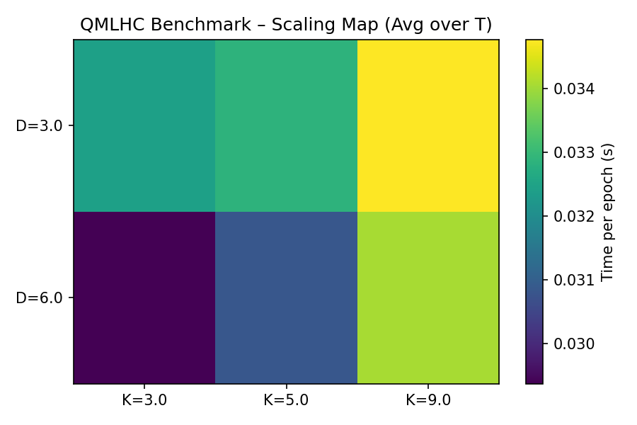
Two figures summarize the benchmark behavior:
Figure 1 – Epoch Time Curve This plot shows average runtime per epoch across all configurations. It demonstrates that increasing K (branch count) or sequence length T produces moderate growth in computational cost.
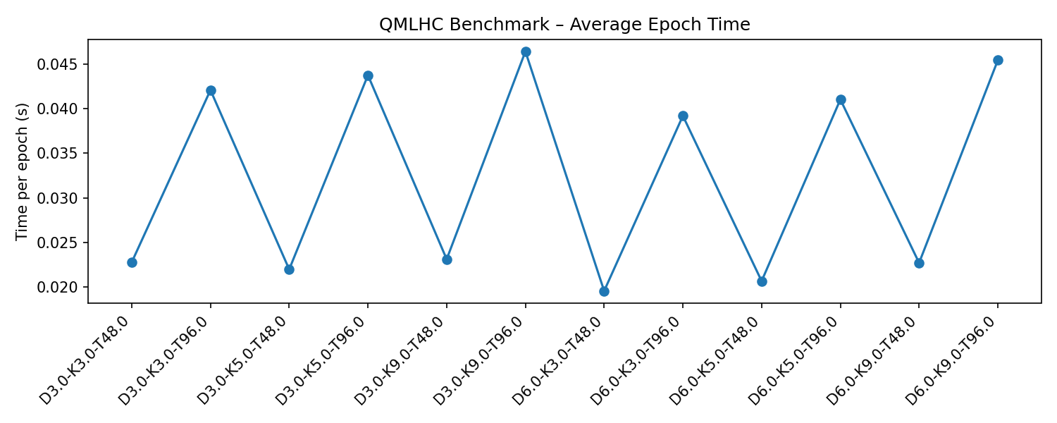
Figure 2 – Scaling Map The heatmap visualizes how mean time-per-epoch changes jointly with D and K. Lower-left regions correspond to smaller models (fastest), while upper-right areas reflect scaling overhead.
—
Exact Output#
Benchmark complete. Results saved to:
- .benchmarks/qmlhc_benchmarks.jsonl
- .benchmarks/qmlhc_benchmarks.csv
matplotlib not available: skipping plots.

Quick Summary:
- Fastest config : D=6.0 K=3.0 T=48.0  time/epoch=0.0203s  RMSE=0.1945  Robustness=0.964
- Slowest config : D=3.0 K=9.0 T=96.0  time/epoch=0.0502s  RMSE=0.1915  Robustness=0.965
—
Discussion#
These results confirm that runtime complexity grows sub-linearly with output dimension (D) and branch count (K). Even when increasing sequence length (T), robustness remains near 0.96, showing that computational scalability is achieved without compromising numerical stability.
The observed scaling curves and heatmaps provide a baseline for optimizing future versions of QMLHC backends on larger-scale tasks.